The second advantage of stacking - increase in bit depth
Stacking astrophotography images will increase signal-to-noise ratio (SNR) by decreasing the noise. The SNR increases as the square root of the number of subexposures that make up the stack. But stacking has a second advantage, that will be especially of use to astrophotographers who use a CMOS camera. These cameras most often have an image output that uses 12 bit of information per channel, as opposed to CCD cameras, which commonly have an image output with 16 bit of information per channel. This means that CMOS cameras represent the entire intensity scale from 0 (lowest) to 1 (highest) in 4096 intensity levels. CCD cameras represent the same intensity scale in 65536 levels. I tturns out that stacking, if done correctly, can increase the bit depth of an image.
Since a continuous intensity scale is represented in discrete value levels, some form of rounding process is needed. In a CMOS camera, fewer levels are used than in a CCD camera, and this can become visible when we stretch an image. In this article I will show how stacking can increase the number of value levels.
For the sake of argument I will use a hypothetical camera which only uses 3 bits of information, or 8 intensity levels (ranging from 0 to 1). While such a camera doesn't seem very practical, we will see that even stacking a relatively low number of images, will dramatically increase the bit depth of the stacked image.
The evidence
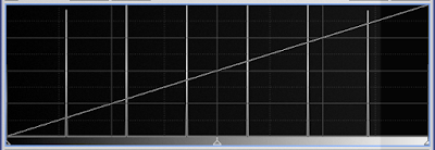
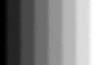
So lets start with the scene we are going to image. It's quite a dull one, consisting of a linear gradient that runs from left (darkest) to right (brightest). Our camera has a sensor of 600 x 400 pixels, and can record only 8 levels of intensity, but the scene, of course has a continuous intensity range.
 |
| Figure 1: the scene |
If we image this scene with our camera, we will get this.
 |
| Figure 2: 3 bit image |
With this output from our camera, we can stack as many images as we want, but the result will always be the same. The camera records the scene in always the same distribution of 8 intensity levels.
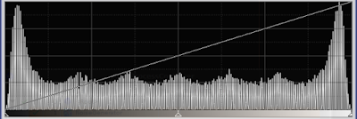
The histogram of this image consists of 8 spikes, representing the 8 intensity levels. Since the zones are all equally wide (except the darkest and brightest), the height of these spikes will be the same.
(The spikes for the darkest and lightest zones are at the very edge of the histogram window, and are difficult to see in this image.)
 |
| Figure 3: histogram |
But what happens when the camera is noisy, and each image ends up like this?
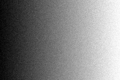 |
| Figure 4: added noise |
This image is the result of adding noise to the noiseless 'staircase' image. The 'width' of this noise is exactly half of the intensity step between each zone. Suddenly, it seems as if the zones have disapeared. So, is this really a 3 bit image? Here's what the histogram looks like.
 |
| Figure 5: histogram |
But wait, shouldn't the histogram of a noisy image show a wider distribution? In this case, no, since we still have only 8 intensity levels. The spatial distribution of the intensity levels is different because of the added noise, but the image is still only represented by 8 levels, or 3 bits of information.
When we get this far, we can apply the first advantage of stacking. Stacking a number of images will decrease the noise in the final image. And, miraculously, this will not bring the original 8 zones back, but a continuous gradient.
Lets stack 32 of these noisy images. We will calculate the average of all 32 values of each pixel position. There will be no pixel rejection. But the final image will be shown as an 8 bit jpeg image. (By the way, all the other images are also 8 bit jpeg images. But since the data only uses 8 discrete levels, the other 248 levels weren't used. That's why the histogram was so 'spikey'.)
 |
| Figure 5: stack of 32 images |
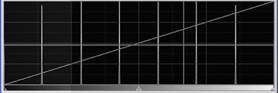
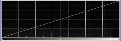
Of course, we can't save this image in 3 bit, but that would give us our 'staircase' image back, just a little noisier. But in 8 bit, we have a nice even gradient. To show how even it is, here's the histogram.
 |
| Figure 6: histogram of the stacked image |
We can see the large number of levels in this image (225 if my calculations are correct), a dramatic increase in bit depth. Ideally, the histogram should be flat, but remember that noise is additive. This means that it is clipped at the low and high end of the histogram. If the noise added to the gradient, gave a negative value, this was clipped to 0 in the camera. And the same happned at the high end. So these areas show a larger number of pixels and a higher peak. The slight unevenness would disappear if we'd used more frames in the stacking process. So how does this work?
The theory
In a noise free world, our 3 bit camera would faithfully register the gray scale of our scene, but only where the intensity of the scene matches the level that the camera can record. In any other position, the intensity is either too low or too high, and the camera electronics will round the value to the nearest digital unit (0 ... 7). That's what makes the staircase. A scene value that falls halfway between two digital units, will either end up rounded up or down. Always in the same manner. However, if we add noise, a pixel value halfway between digital units will sometimes end up being rounded up, and sometimes being rounded down. Depending on the value and how much noise we add, it will end up more in the lower or more in the higher digital unit. If we only have two frames to stack, then an intensity value halfway between two units, can one time be represented by the lower unit, and in the other frame by the higher unit. The average value will then be the average of the two units. If we had a one bit camera, which only can register 0 (black) or 1 (white), an intensity value of 0.5 with some added noise, can end up 0 in one frame, and 1 in the other, with a 50% chance. The average will then be 0.5.
If we have three frames in our stack, the pixel values can consist of two 0 and one 1, or one 0 and two 1. We can register the intermediate values 1/3 and 2/3, as well as the values 0 and 1. We now have 4 intensity levels which we can resolve. If we continue adding frames to our stack, then each added frame will add one more intermediate level of intensity in our stacked image. If two frames add one level, three frames add two levels, and four frames add three levels (1/4, 1/2, 3/4), then 32 frames add 31 levels between each existing level. The new image should have 32\cdot7+1=225 levels. This of course, applies only if our stacked image can hold all those levels of intensity. We need 8 bits to represent each intensity level.
In most cases, the average and median of a data set will follow each other closely, if we have enough data. So let's look at what happens when we use median stacking rather than average stacking. We can actually predict what will happen. In a stack of any odd number of frames, the actual pixel value of the stacked image will be a pixel value of one of the images that went into the stack. This predicts that any pixel value in the stacked image will be one of the seven original levels. There should be no improvement in bit depth if we use median stacking. Well, here's the result of median stacking. The same images that went into the average stack were used.
 |
| Figure 7: median stacking |
Apart from noisy transitions, we still see eight intensity levels. If we examine the transitions closely, there are some pixels where we actually have recorded a value midway between two levels, but this is due to the way the median is calculated for an even number of samples. If we add or remove one frame, the intermediate levels will dissappear. Here's the histogram of our even numbered stack.
 |
| Figure 8: histogram of median stacking |
Finally, let's see what happens when the noise in the recorded image not quite obliterates the staircase appearance in each image. We halve the noise in each image, which now looks like this.
 |
| Figure 9: half the noise in each image |
There's still some of the staircase left, and the stacked (averaged) image looks like this.
 |
| Figure 10: average stacking with half the noise |
While this certainly is an improvement, there are still annoying bands left in the final image. It seems that for a good result, we actually need enough noise to really obliterate the bands in the original image. The width of the noise should be at least half a digital unit. Anything less will not give us the smooth image we want.
Summary
Let's summarise. It is possible to increase the bit depth of an image by stacking noisy images. The noise must be sufficient to obliterate the staircase effect in the images that make up the stack. You have to use average stacking for this to work, and you have to be able to save the result in a format that keeps the higher bit depth. Stacking an 8 bit image, and saving it in an 8 bit format, will not do you any good. In the same way, stacking 16 bit images and saving the result in 16 bit format will not achieve anything. But even a moderate number or images in 12 bit format, can give you a 16 bit result.
This method works, because noise will destroy the banding that occurs in low bit depth images, and stacking will reduce the noise in the final image.
The proof of this is in the proverbial pudding. Here's an image of a little more than a gradient. Added noise and 3 bit depth.
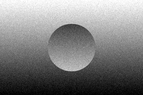 |
| Figure 10: a noisy image in 3 bit |
And this is what a stack of 32 of those reveals. Impressive, isn't it? (If you're not impressed, look closely at the lower left corner. Still not impressed?)
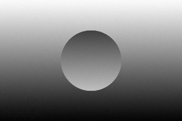 |
| Figure 11: 32 images stacked |


Inga kommentarer:
Skicka en kommentar