Optimising offset for the ASI 174MM-Cool

Used last night's cloud cover to do some testing with my cooled CMOS, the ZWO ASI 174MM-Cool.
The gain of CMOS cameras is variable, and to avoid clipping dark pixels, you have to add an offset or pedestal. Basically this means that each pixel value that is read is transformed by an amplifier and analog - digital converter (ADC) according to the formula

ADU = (pv + Offset)/Gain

The odd use of dividing by gain in stead of multiplying is because gain is defined as e/ADU. One would also expect the offset to be in ADU, giving the formula

ADU = pv/Gain + Offset

But I found that at high gain setting, any change in offset is much more critical than at low gain, so I think the proper formula is the first one.

First off, you have to distinguish between gain setting ( for the ASI 174, the gain setting can be varied from 0 to 400) and real gain (about 8 e/ADU at setting 0, 1 e/ADU at setting 189, and decreasing e/ADU the higher the setting goes).

I used this simple method to determine the best offset for various gain settings.

I took one bias frame at the shortest possible exposure time (32 microseconds) for each gain/offset combination. I varied the gain setting from 0 to 400 in 100 unit steps, plus unity gain (gain setting 189). I then varied the offset and used PixInsight image statistics to determine when the lowest pixel value (in ADU) started to increase. For some reason the lowest pixel value was at least 1, so I increased offset until I got >2 - 3 ADU as a minimum pixel value.

I did the tests at -15 degrees Centigrade, because that is the temperature I use for imaging at the moment. Offsets shouldn't be that temperature dependent any way.

The highest offset that my driver (INDI) allows is 240, which wasn't high enough for a gain setting of 400. The highest gain setting that can be used with the offset at 240, is about 365.

This exercise shows that in order to achieve the highest dynamic range in the ASI 174MM, you can optimise the offset for each gain setting to avoid pixel clipping. Using a higher offset than needed to avoid clipping will decrease the dynamic range of the camera.

That other reason to stack images - increase in bit depth

The second advantage of stacking - increase in bit depth

Stacking astrophotography images will increase signal-to-noise ratio (SNR) by decreasing the noise. The SNR increases as the square root of the number of subexposures that make up the stack. But stacking has a second advantage, that will be especially of use to astrophotographers who use a CMOS camera. These cameras most often have an image output that uses 12 bit of information per channel, as opposed to CCD cameras, which commonly have an image output with 16 bit of information per channel. This means that CMOS cameras represent the entire intensity scale from 0 (lowest) to 1 (highest) in 4096 intensity levels. CCD cameras represent the same intensity scale in 65536 levels. I tturns out that stacking, if done correctly, can increase the bit depth of an image.

Since a continuous intensity scale is represented in discrete value levels, some form of rounding process is needed. In a CMOS camera, fewer levels are used than in a CCD camera, and this can become visible when we stretch an image. In this article I will show how stacking can increase the number of value levels.

For the sake of argument I will use a hypothetical camera which only uses 3 bits of information, or 8 intensity levels (ranging from 0 to 1). While such a camera doesn't seem very practical, we will see that even stacking a relatively low number of images, will dramatically increase the bit depth of the stacked image.

The evidence

So lets start with the scene we are going to image. It's quite a dull one, consisting of a linear gradient that runs from left (darkest) to right (brightest). Our camera has a sensor of 600 x 400 pixels, and can record only 8 levels of intensity, but the scene, of course has a continuous intensity range.

Figure 1: the scene

If we image this scene with our camera, we will get this.

Figure 2: 3 bit image

With this output from our camera, we can stack as many images as we want, but the result will always be the same. The camera records the scene in always the same distribution of 8 intensity levels.

The histogram of this image consists of 8 spikes, representing the 8 intensity levels. Since the zones are all equally wide (except the darkest and brightest), the height of these spikes will be the same.

(The spikes for the darkest and lightest zones are at the very edge of the histogram window, and are difficult to see in this image.)

Figure 3: histogram

But what happens when the camera is noisy, and each image ends up like this?

Figure 4: added noise

This image is the result of adding noise to the noiseless 'staircase' image. The 'width' of this noise is exactly half of the intensity step between each zone. Suddenly, it seems as if the zones have disapeared. So, is this really a 3 bit image? Here's what the histogram looks like.

Figure 5: histogram

But wait, shouldn't the histogram of a noisy image show a wider distribution? In this case, no, since we still have only 8 intensity levels. The spatial distribution of the intensity levels is different because of the added noise, but the image is still only represented by 8 levels, or 3 bits of information.

When we get this far, we can apply the first advantage of stacking. Stacking a number of images will decrease the noise in the final image. And, miraculously, this will not bring the original 8 zones back, but a continuous gradient.

Lets stack 32 of these noisy images. We will calculate the average of all 32 values of each pixel position. There will be no pixel rejection. But the final image will be shown as an 8 bit jpeg image. (By the way, all the other images are also 8 bit jpeg images. But since the data only uses 8 discrete levels, the other 248 levels weren't used. That's why the histogram was so 'spikey'.)

Figure 5: stack of 32 images

Of course, we can't save this image in 3 bit, but that would give us our 'staircase' image back, just a little noisier. But in 8 bit, we have a nice even gradient. To show how even it is, here's the histogram.

Figure 6: histogram of the stacked image

We can see the large number of levels in this image (225 if my calculations are correct), a dramatic increase in bit depth. Ideally, the histogram should be flat, but remember that noise is additive. This means that it is clipped at the low and high end of the histogram. If the noise added to the gradient, gave a negative value, this was clipped to 0 in the camera. And the same happned at the high end. So these areas show a larger number of pixels and a higher peak. The slight unevenness would disappear if we'd used more frames in the stacking process. So how does this work?

The theory

In a noise free world, our 3 bit camera would faithfully register the gray scale of our scene, but only where the intensity of the scene matches the level that the camera can record. In any other position, the intensity is either too low or too high, and the camera electronics will round the value to the nearest digital unit (0 ... 7). That's what makes the staircase. A scene value that falls halfway between two digital units, will either end up rounded up or down. Always in the same manner. However, if we add noise, a pixel value halfway between digital units will sometimes end up being rounded up, and sometimes being rounded down. Depending on the value and how much noise we add, it will end up more in the lower or more in the higher digital unit. If we only have two frames to stack, then an intensity value halfway between two units, can one time be represented by the lower unit, and in the other frame by the higher unit. The average value will then be the average of the two units. If we had a one bit camera, which only can register 0 (black) or 1 (white), an intensity value of 0.5 with some added noise, can end up 0 in one frame, and 1 in the other, with a 50% chance. The average will then be 0.5.

If we have three frames in our stack, the pixel values can consist of two 0 and one 1, or one 0 and two 1. We can register the intermediate values 1/3 and 2/3, as well as the values 0 and 1. We now have 4 intensity levels which we can resolve. If we continue adding frames to our stack, then each added frame will add one more intermediate level of intensity in our stacked image. If two frames add one level, three frames add two levels, and four frames add three levels (1/4, 1/2, 3/4), then 32 frames add 31 levels between each existing level. The new image should have 32\cdot7+1=225 levels. This of course, applies only if our stacked image can hold all those levels of intensity. We need 8 bits to represent each intensity level.

In most cases, the average and median of a data set will follow each other closely, if we have enough data. So let's look at what happens when we use median stacking rather than average stacking. We can actually predict what will happen. In a stack of any odd number of frames, the actual pixel value of the stacked image will be a pixel value of one of the images that went into the stack. This predicts that any pixel value in the stacked image will be one of the seven original levels. There should be no improvement in bit depth if we use median stacking. Well, here's the result of median stacking. The same images that went into the average stack were used.

Figure 7: median stacking

Apart from noisy transitions, we still see eight intensity levels. If we examine the transitions closely, there are some pixels where we actually have recorded a value midway between two levels, but this is due to the way the median is calculated for an even number of samples. If we add or remove one frame, the intermediate levels will dissappear. Here's the histogram of our even numbered stack.

Figure 8: histogram of median stacking

Finally, let's see what happens when the noise in the recorded image not quite obliterates the staircase appearance in each image. We halve the noise in each image, which now looks like this.

Figure 9: half the noise in each image

There's still some of the staircase left, and the stacked (averaged) image looks like this.

Figure 10: average stacking with half the noise

While this certainly is an improvement, there are still annoying bands left in the final image. It seems that for a good result, we actually need enough noise to really obliterate the bands in the original image. The width of the noise should be at least half a digital unit. Anything less will not give us the smooth image we want.

Summary

Let's summarise. It is possible to increase the bit depth of an image by stacking noisy images. The noise must be sufficient to obliterate the staircase effect in the images that make up the stack. You have to use average stacking for this to work, and you have to be able to save the result in a format that keeps the higher bit depth. Stacking an 8 bit image, and saving it in an 8 bit format, will not do you any good. In the same way, stacking 16 bit images and saving the result in 16 bit format will not achieve anything. But even a moderate number or images in 12 bit format, can give you a 16 bit result.

This method works, because noise will destroy the banding that occurs in low bit depth images, and stacking will reduce the noise in the final image.

The proof of this is in the proverbial pudding. Here's an image of a little more than a gradient. Added noise and 3 bit depth.

Figure 10: a noisy image in 3 bit

And this is what a stack of 32 of those reveals. Impressive, isn't it? (If you're not impressed, look closely at the lower left corner. Still not impressed?)

Figure 11: 32 images stacked

Handling Fits files in batches - FITSFileManager in PixInsight

Lately I have processed a number of images taken with the Liverpool Telescope on La Palma. The images in their archives are FIT files that have a large header with all the information you'd ever want on the image. When downloaded, the iamges need to be extracted (from tar or tgz formats) and sorted. When I started out with this I would download the images from each filter separately, in order to keep the colour channels apart, but this gets tiresome. Lately I have started to use a script in PixInsight that does the work for me. Here's how I do it.
I download all the images at once and put them in one folder on my computer. Then I extract the images from the compressed tar-files. Next I start the FITSFileManager script in PixInsight (Scripts -> Utilities). I rename the image files, using the FILTER keyword as a prefix to the filename. The file name template is: '&FILTER1;_&filename;'. I move the files to the same directory as where they were stored, so that the new file name replaces the old file name. This way, my files are easily sorted and identified.

Contour mask in PixInsight - an alternative way

If you want to reduce stars in PixInsight, you need a contour star mask. The StarMask process has this option, and for many images this works just fine. But occasionally I find it difficult to make this mask work for both large and medium sized stars. Here's an alternative to the standard method.
Use StarMask to create a standard star mask. Choose the number of layers large enough to include even large stars. To get this to work, you may need to decrease the noise threshold a bit. On most of my images, I start with 6 or 7 for the number of layers, and about 0.35 for the noise threshold. But really it depends entirely on your image and what size stars you have. Keep the structure parameters at their default values (Large = 2, Small = 1, Compensation = 2)
When you're satisfied with the mask, create another one, but decrease the number of layers by one, and set the structure parameters to 0.
Now, use PixelMath to subtract the second mask from the first. If you want to keep the original masks, create a new image. Otherwise use the expression '$T - star_mask2' and apply it to the first mask (with the larger stars). The star mask should now show donuts for stars. If the donuts don't open up (ie still gray or white in the center), you need to increase the intensity of the second mask by using the HistogramTransformation tool. Occasionaly, I have had to use the CloneStamp tool for a tricky star or two. Just take a sample from the black background and clone it in the white star that is reluctant to open up. Just make sure you put it in the right spot, otherwise you may end up with a lopsided star.
When you are satisfied with the contour shapes, you can increase the intensity of the mask with the HistogramTransformation tool, and blur the mask with the Convolution tool.
The advantage of this method is that it creates contour masks for large and small stars alike, while the standard method, sometimes fails to create contours for smaller stars.

star repair in PixInsight - part 2

While reprocessing old data, I came across a very instructive incidence of star over exposure. When imaging under light polluted skies, sky glow is added to any sky signal (stars, nebulae, etc). If the pollution is strong enough to over expose stars, the true star colour data is destroyed. When the sky glow is removed during post processing, this will lead to bright stars having the wrong colour.
For example, say a bright star is slightly blue in colour. Without any sky glow, it would register as RGB 0.8, 0.8, 0.95. Sky glow gives an added 0.3 in blue. This will put the star colour on sensor as RGB 0.8, 0.8, 1.0, since the maximum value for a pixel is 1.0.
When the sky glow is removed during background extraction, the value 0.2 will be subtracted, and we end up with a star's RGB values of 0.8, 0.8, 0.7. The star core has suddenly turned yellow. However, away from the core, the star will still be blue, since these areas weren't over exposed. Therefore the need to correct star colours.
During normal stretching of an image, most of the bright stars will be maximised, and have a final colour of RGB 1.0, 1.0, 1.0. However, if masked stretch is used, the stars will not be saturated, and will have a funny looking core.
Here's an example of an unstretched star, with (left) and without (right) colour repair.

When should star repair be implemented in the workflow?
Of course, before any stretch is applied, the colour must be corrected. However, there is one earlier instance where star colour matters in processing, and that is during colour calibration.
Colour calibration tries to set a white point by looking at all the stars in an image, and apply a calibration scheme that is determined by the average star colour. When the star colour is wrong due to over exposure and background extraction, the white balance after colour calibration will be off. Therefore, there is an argument for applying HSV repair prior to colour calibration. The workflow then becomes as follows:

• cropping of edges
• background extraction (ABE or DBE)
• background neutralisation
• HSV repair
• colour calibration

This image shows the effect of doing HSV repair before (left) or after (right) colour calibration. Due to the skyglow adding mainly blue to the image, several star cores had a warmer colour after DBE. This resulted in the colour calibration routine making the blue stars more intense blue. By doing the HSV repair process prior to colour calibration, stars got a more natural blue colour after stretching.

star repair in PixInsight

When stars start to get over exposed during data collection, their core may become a different colour than the normally exposed outer halo. When the stacked image is stretched using MaskedStretch in PixInsight, stars are stretched less than dimmer parts. This means that stars in the stretched image are not saturated, and can display an odd colour. PixInsight has a script that can correct star cores of partially saturated stars. It is called "Repaired HSV Separation", and can be found under Scripts -> Utilities. The script should be applied just before the first stretch. It will decompose the colour image into H, Sv, and V colour components, and repair the colour values of the stars.
The different components are then to be combined using the ChannelCombination process (which is under ColorSpaces).

The upper part of the dialog box is used to determine which images are to be created, while the lower part is used for repair of the H, Sv, and V channels.For best results, mainly the Repair level parameter needs to be adjusted.
Alejandro Tombolini (who brought this script to my attention), recommends to use the unrepaired V channel when combining the channels. But experiment to find out if the repaired or unrepaired V channel works best. Be sure to select the HSV colour space.

Here's how it affected one of my most recent images, a before and after shot of the Pleiades (M45). Look at the core of the brightes stars. In the original image, the cores arepink in colour, while in the repaired image, they are blue, the same colour as the outer haloes.

Correcting dark lines in dslr astro images

My Pentax DSLR suffers from dark horizontal lines when I photograph bright stars. I'm not sure about the cause of this, but it may be some reverse blooming or ADC related issue. This issue isn't uncommon for digital cameras, but it sure is a nuisance.

Alejandro Tombolini showed in one of his processing examples how to deal with these lines. Here's my adaptation of his process.

I will use the CanonBandingReduction script to correct the lines. This script works only on entire images, and can introduce an uneven background and other artefacts when used on images which do not have bands across the entire width.
I therefore start with making a preview that contains the area I want to correct. I leave some margin, because later on I will clone the preview and shrink the clone.
By dragging the preview onto the workspace, I create a new image, which I apply the CBR script on.
The next step is to make this preview the same size as the original image. For this I use the crop tool.

Set the margins such that the image becomes the correct size, with the corrected image now in the same place as the preview in the original. If the result is ok, the image is saved as xisf file.

Next I shrink the preview in the original image and create a hole in the image where the preview is. For this I use pixelmath.

A new image is created with a black patch where the (smaller) preview was.
This image is also saved.

Finally the two saved images (the corrected preview, and the uncorrected image with the black patch) are merged using GradientMergeMosaic.

And this is the corrected image

Removing hot pixels in a stacked image

Sometimes even an aggressive hot pixel filter won't remove all hot pixels. Here's a technique that can remove any residual hot pixels in a final stacked image. I use PixInsight's Morphological Transformation with a starmask to remove these nuisances.
Here's a crop of an image, showing what I'm talking about. The image was taken with a DSLR and consists of a stack of 10 sub frames exposed for 15 minutes each at ISO 800. My camera, a Pentax K20D, is getting old, and I always have lots of hot pixels in my images. Calibration removes most, but frequently a number remain after image integration. The technique which I describe here will dim the remaining pixels.

hot pixels after stacking

I start with making a Luminance copy of the image in its linear state, and apply STF to this grayscale image. Then I use the StarMask tool with a low value for Scale (typically 3 works ok) and a noise threshold of 0.5 (to be experimented with). I decrease large-scale, small-scale and compensation (1, 0, 1) and smoothness (about 6 - 8). Then apply the mask tool to the luminance copy. It may be necessary to tweak the parameters. No stars should be in the "Star-Mask" that is created.
When I'm satisfied, I apply the mask to the original colour image.
For pixel removal I use Morphological Transformation with Morphological Median as operator. Amount to about 0.5, iterations to 4 - 5, and Structuring Element to 9 pixels with a circular pattern.
Apply the tool to the image. If hot pixels of a certain colour remain, I split the RGB channels and use the channel that has the remaining hot pixels to repeat the process. The result is this.

Same crop after hot pixel removal

Further tweaking of the star mask and morphology parameters can improve this result even more, of course.

Creating a customized "Batch Process" in PixInsight

Some processes in PixInsight are adapted for large batches of images. But sometimes you want to do a sequence of process steps, for which there is no batch process, on several images. Opening each image and applying a number of processes is quite tedious.
Fortunately, PixInsight has a solution for this. It involves an image container and a process container.
For any process in PI, if you drag the small triangle in the lower left corner to an image, it will apply that process to the image. This can also be applied to a collection of images, if these are in an image container. And the process doesn't have to be a single process, it can be any number of processes that are in a process container. How is this done?

Prepare the process container.

Open an image and apply the processes you want to batch to that and other images.
Now open the image's history explorer, which should be located on the left edge of the workspace. Drag the small triangle at the bottom left to an open area in the workspace. This will create an instance of the process history of that image as a process container in the workspace.

Now you can close the image without saving.

Create an image container

 Next create an image container by right clicking anywhere in the workspace, or press Ctrl+Alt+I.

This will create an image container in the workspace. Open the container and add the image files you want to batch process. Also supply a name for the output directory where you want the processed images to be saved. Finish by dragging the small triangle to an empty spot in the workspace. This will create a new instance of your image container, with all the images in it.

Apply the processes in the process container by simply dragging the process container onto the image container that contains the images.
That's it. You've just applied several process to a batch of images.

First experience with INDI on Raspberry Pi - part 2

Last week , when I tried to control my mount through indi on a Raspberry Pi, I managed to install the server and connect from my laptop to the indi server on the RPi. However, the mount didn't respond. It turned out that the USB serial cable didn't work anymore.
Yesterday I received an EQDIR cable from FLO, and connected it to the mount. After some adjustment of the parameters in linux and the Indi client, it all worked perfectly.
Now I can control my mount from PixInsight or any client that can run the indi protocol.
The next step will be to install and test servers.
Short recap of the installation so far.

1. Install an Ubuntu Mate image on a SD card for the RPi
2. Connect the RPi to the home Wifi network and set parameters to connect to PuTTY
3. Connect to the indi repository, download and install the indi server
4. Set $USER for dialout permission
5. Create a permanent USB entry for the connector
6. Start the server
7. Start the client and connect to the server
8. Configure the site and the mount in the client

So far PixInsight can connect to the mount and send goto commands. With the search capability, I can just search for say, M27 and the mount will slew to it.
Of course, this assumes that the mount is aligned, and so far PixInsight can't do a 2-star alignment.
I just hope that this will be implemented soon.
For the time being, my intended workflow is as follows.

1. Haul out the mount and set up
2. Level mount
3. Start mount with SynScan
4. Do a polar and a 3-star alignment
5. Park the mount and power off
6. Disconnect the SynScan
7. Connect the RPi and boot
8. Connect the client

Further testing is delayed by clouds :-(

Note on Dynamic Background Extraction

Astroimages allmost always have a background gradient that needs to be removed. Gradients can have two basic causes; either they are due to limitations of the optical system (vignetting), or to uneven illumination of the night sky. Most of us live and photograph in light polluted environments, and our astroimages incorporate stray light from street lamps or city lights. Even when photographing from a dark site, there is the inevitable sky glow. Whatever the cause of an uneven background, it is seldom something we want incorporated in our images.
PixInsight has two processes for gradient removal; Automatic Background Extraction (ABE) and Dynamic Background Extraction (DBE). These two processes work slightly different from each other, so it is a good thing to know them both. ABE is an automatic process, that does most of the work for you, especially the more laborious part of placing samples in the image. DBE on the other hand, allows for more user control.
In this article, I intend to give my experience of the DBE process, and how I use the various settings in the DBE control window.
Shortly, what you do with DBE is take samples of the background in your image and create a model of the image background, based on those samples. (Note that I assume you are working with an RGB colour image.)



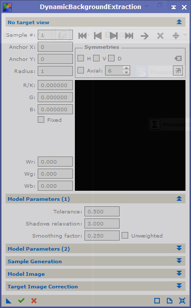
Dynamic Background Extraction

When you open the DBE process (Process | BackgroundModelization | DynamicBackgroundExtraction), you start with connecting it to an image, the target,  in your workspace. This is done by either clicking in the image you wish to connect to, or clicking the reset icon at the bottom right of the control window (the four arrows pointing inwards). The latter option will also reset all settings in the control window. The active image is now linked to the process and it shows the symmetry lines that can be used by DBE. More on the symmetry lines in a moment.

Target View

Each time you click in the target window, a new sample will be created at that position. In the target view you will see how individual pixel values will be used in the creation of the background model. Each sample has a position (anchor x, y) and a size (radius). The square field in the target view panel shows how each pixel is used in the model. This field should ideally consist of only bright pixels. If the pixels have a colour, than the pixel will only be used in the calculation of the model for that colour. The three values Wr, Wg, Wb are the weights in red, green and blue for the combined pixels in the sample. They determine how much this sample will contribute to the background model. In this view you can also determine if symmetries are to be used. If you have an image which you know has a symmetrical background (vignetting for example), then you can create samples in one place where the background is visible, and use those samples in other parts of the image, even if the background there is not visible. When you click on one of the boxes (H for horizontal, V for vertical, D for diametrical), a line will show where the sample will be used. Not that you can control the symmetry for each individual sample. Use with care.

Model Parameters

In this panel you will set how strict your model is going to be. The most important value is Tolerance. Increase this if you find that too many samples are rejected. The default is 0.5, but expect to use values up to 2.5 regularly, and in extreme cases even higher than 5 - 7. But try to keep this value as low as possible. Once you have created all your samples, and are satisfied with where you placed them, you can decrease this value somewhat and recalculate the samples, until samples are being rejected. Choose the lowest value you can get away with, as this will result in a better approximation of the true background.
Smoothing factor determines how smooth your model is going to be. If you set this to 0.0 then the background will follow your samples very strictly. Increase this value to get a smoother background model if you see artefacts in the model.

Sample Generation

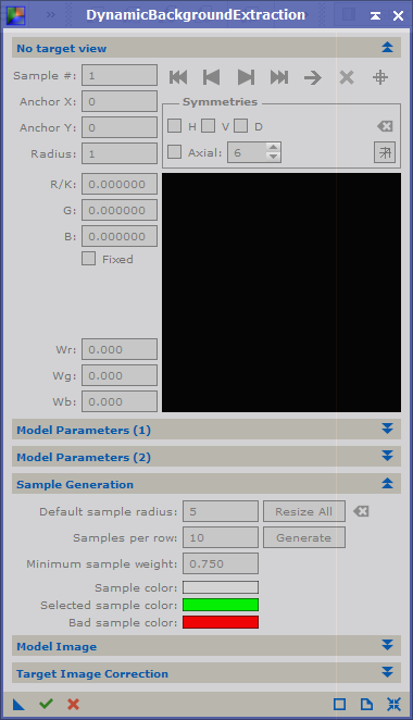
DBE Sample Generation

DBE lets you create your own samples, which is great if you have an image with lots of stars or nebulosity, but it can also create samples for you.
The first parameter sets the size of the samples. The samples will be squares with "sample size" number of pixels on either side. Use the largest samples that will not cover any stars. Obviously, if you have an image of the milky way, you will need to keep this value small, or you won't be able to position samples without covering stars.
Number of samples determines the number of samples that will be created across the image. It is generally best to use more samples. If you use to few samples, your background model may not represent your true background. Even if you have a linear background, you can model it with many samples. On the other hand, if you have a more complicated background, you can't model it with say three samples.
Minimum sample weight is only important if you let the process create samples. If you know that you have a strong gradient in the background, you should decrease its value to maybe 0.5 in order to create more samples. This parameter is used with Tolerance, to create samples in areas with more gradient.

Model Image

This is where you can set how your model background will be represented as an image. This is probably the least important panel. No comments on this panel.

Target Image Correction

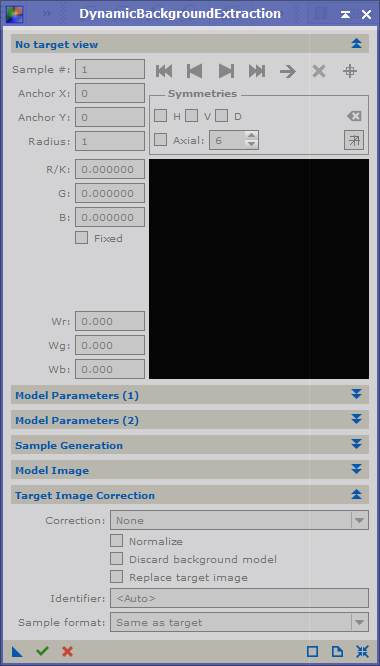
DBE Target Correction

This is probably the most important panel, as it is here you determine which type of gradient you want to remove. There are three options for gradient removal; none, which you would use to test settings without applying the process to your image; subtraction, which is used to remove gradients from light pollution or sky light; and division, which is used to remove gradients caused by the optical system.
Examine your image and determine the most likely cause of the gradients. If you find that you have gradients due to both vignetting and light pollution, you may have to apply the DBE process twice, but in many cases once is enough. If you need to apply DBE twice, it seems most logical to get rid of vignetting first, since it has affected all light entering your imaging setup. You would then first apply division as your correction method, and secondly apply subtraction with a new DBE process.
You can choose to view your background model, or to discard it. I always leave this option unchecked, since I want to examine my model. This is handy in case you want to refine your samples and settings. If you find that the model looks complicated, blotchy and with several colours, then you are probably overcorrecting. This may result in the loss of colour in nebulas. Make it a habit to check the background model before you discard it.
You can also choose to replace your image with the corrected version, or to create a new image. If you choose to create a new image, then that will not have any history. On the other hand, if you replace your original image, you keep its entire history. This can be handy.

How stars are handled in DBE

(This is the way I understand it works, which may be wrong)
If you place a sample over a star, you will notice that the sample will show a hole (= black) at the star position, with probably a colours band around this hole. This means that the pixels that represent the star, have a weight = 0, and will not be considered in the background model. However, the coloured band can be a halo or chromatic abberation, and the pixels will  be taken into account for the background model. To avoid this, it is always better not to place samples over stars. If you can't avoid this, then at least examine the sample carefully, and try to place it such that it's effect is minimized. Also note that since the position of the star is not taken into account, the sample consists of fewer pixels, and each pixel will have a larger contribution for the background model.

On the size and number of samples

The samples you create should represent true background. If your image has large patches of background, you can have larger samples. If on the other hand, your image has lots of nebulosity or lots of small stars, then the background will only truly be covered by small samples. Examine your image and set sample size accordingly.
Should you use few or many samples?
It seems that some people like to use few samples in an image, while others use smaller but many samples.
There is a danger that if you use many samples, some will cover nebulosity. When the correction is applied, this will lead to destruction of the target.
On the other hand, if you only place a few samples, these may not pick up the variation of the background properly.
As usual, the number of samples that you should use must depend on the image.
Theoretically, if you have a linear gradient in an image, creating just two samples would be enough to model the background. But any mistake in either of the samples will have a severe effect on the accuracy of the background model. If you use a larger amount of samples, then each individual sample will have less effect on the background model. This generally results in a better model than using just a few samples.
I have had success with using a large number of samples (20 - 25 per row, or some 400+ samples) in my images. It does however, take quite a while to place all these samples. Even if I automatically generate the samples, I still have to make sure that they don't cover stars or part of my target.
One method that I have found helpfull is to create a clone of the image that is then stretched. This allows me to see where samples can be placed, and where they should be avoided. I then place the samples on this clone, but do not apply the correction.
After placing the samples, I create a process instance on the workspace and delete the open instance. I then apply the process on the unstretched original image.

What to look for after background extraction

As I already mentioned, I always keep the extracted background image. I examine this, and if I find that the background contains traces from nebulosity, I generally undo the extraction and change the samples in my image.
I also examine the corrected image for artefacts. If samples are too close to a target or a star, there is a chance that DBE creates a dark region around this target or star. Even in this case I undo the operation and move or remove samples.
I repeat this process until there are no dark patches left where they shouldn't be, and the background looks smooth while nebulosity has been preserved.
It can take quite a while to get the extraction right, but it will make further processing easier if you spend more time on this step.

first experiences with INDI on Raspberry Pi

Now that I have invested in a proper mount, I'm also looking into remote (15 meters) operation of it.
I don't want to drag my laptop out into the garden just to have it covered with dew, and I like the size of Raspberry Pi. This, and the fact that PixInsight is moving into the direction of hardware control through the INDI protocol, made me decide to look into the INDI solution, rather than EQMOD.
So, last weekend I erased my Pi memory card and installed Ubuntu Mate. This OS was recommended on the INDI website (indilib.org ).
Now, I have very little experience with linux, and for most of the things I do, I need to follow a tutorial or google my way around. The following is probably not the best way to do it, but these are my experiences.

Installing the OS wasn't much of a problem; download and extract the image. Then use Win32DiskImager to write the OS image onto the memory card.
Started the OS, and managed to connect it to PuTTY, but in the beginning I mainly used the desktop and a terminal window in the desktop.
Installing the INDI library took some time. For some reason I couldn't register or connect to the INDI repository (mutlaqja ppa), and the desktop on several occasions reported an internal error. Finally (don't aks me how) I managed to connect to the repository and install INDI. To get this far took quite a while so I read the OS image back to windows. I figured that if I ever need to go back and reinstall the OS, at least I won't need to do it from scratch.
I managed to get INDI server up and running, and decided to rename the USB port for permanent reference. Some googling gave the answer, and some more tapping away on my keyboard (now I don't use Mate anymore, but am connected through PuTTY and WiFi).
I then connected the mount through Synscan's serial cable and a serial/usb interface.
I managed to connect from PixInsights INDI client, but the program crashed a few times. Again, don't ask me why. I have never been able to crash PixInsight, but during the past few days I managed it twice. (Mind you, I have managed to bring it to it's knees by integrating some 200+ 14 Mpixels drizzled images. But that's a different story.)
It seems that there isn't a "hello world" application that lets you test a partial setup. There isn't even a proper tutorial that covers a complete setup. It takes some googling and looking around the INDI website to get ideas and suggestions for solutions.
Anyway, I also tried connecting through Stellarium, which didn't protest and connected to the server.
Both the PI and Stellarium connections worked fine, as the server kept responding to slew requests. However, the mount didn't budge an arcsecond.
After a long time installing, uninstalling and reinstalling various things and starting and stopping the server, rebooting the RPi, etc, etc, I finally called it a night, not having moved the mount remotely at all.
I dismantled the RPi, cables, and the mount (I'm doing this more or less in the family living room), and just as I was about to disconnect the serial cable, I noticed that neither of the LEDs was lighting or blinking.
It appears that my serial/USB connecter isn't working anymore. So now I'm waiting for the HITECH EQDIR Synscan/USB interface to arrive from Firstlightoptics.
Since everything else worked fine, just plugging in the connector should make the remote setup work. Something tells me though, that it will not work from the start, even with a new cable.

The setup sofar:
RPi 2 with Ubuntu Mate, connected to PuTTY on Windows.
sudo apt-add-repository ppa:mutlaqja/ppa (works after a few tries and reboots)
sudo apt-get install indi-full
sudo adduser $USER dialout (so I don't have to be root user to use indi)
create a rules file to rename the mounts usb port, using udevadm
indiserver -m 100 -v indi_eqmod_telescope
several reboots along the way.

To do next:
Make sure that the new connector works (without the Synscan)
Make sure that the setup works (mount connected to RPi without the Synscan inbetween; indisverver controlled by Stellarium on Windows machine)
Make sure that indiserver starts up automatically after booting the RPi.
Find and install a client that lets me control the mount and will replace the Synscan.

To be continued, I guess.

PixInsight process icons

When you process an image, it's always handy to copy the processes you use to the workspace. You can do this by dragging the little triangle in the lower left corner onto the workspace. This will preserve the settings for that instance.
The only problem with this is that all process icons get a name ProcessXX, where XX is a number.
It is easy to change this name to something more sensible:
Click on the small N on the right hand side of the icon. This will open a dialog box where you can change the icon name. If you want to add a description, you click on the small D. Use this for example to write which mask you used for the process.

process and image icons

Image icons have no description, but you can change their name. Also note that process icons are full rectangles, while image icons have one corner missing.

Noise reduction for DSLR astro images

Astro images taken with a DSLR at a high ISO setting are noisy, and the best way to decrease the noise level is of course to take lots of images and stack these. But even then, some sort of noise reduction is necessary.
Noise in DSLR images manifests itself as intensity noise and colour noise. Think of it this way; noise is a random variation in pixel values. Pixel values can either vary in intensity, more or less intensity of the same colour, or in colour, same intensity but another colour. Both these variations have to be addressed by a noise reduction process.
Here I will show you my procedure for DSLR images.
First I apply noise reduction to the luminance or lightness (colour intensity) of the image, and then a very aggresive noise reduction to the chrominance (colour variation).
One of the most efficient luminance noise reduction methods in PixInsight is TGVdenoise. This method is especially good at reducing high frequency (or small scale) intensity noise, and is based on a diffusion algorithm. This means that it detects variation in pixel values and pushes these variation outwards, away from the pixel. As in any diffusion process, the longer you let the process continue, the stronger the spreading process will be. In the case of TGVdenoise this means that you let the process go through many iterations.

One of the best ways to use TGVdenoise was devised by Philippe Bernard. A presentation in french can be found on his website; TGVDenoise. A slightly updated version was presented on the PixInsight forum by member Tromat.
(Always have a  STF stretch applied to the image. This keeps the image in its linear state, but allows you to see on screen what the image looks like. Also, always test the settings on a small preview that contains both background and a weak signal you want to preserve.)



Before and after luminance noise reduction, using TGVdenoise

The second stage of noise reduction is to reduce colour noise, or chrominance noise. For this I use the MultiscaleMedianTransform.
In the noise reduced image, you will probably still see colour variation in the background. MMT will take care of this noise.
First you will need to create a mask that will protect the stars and target.
For this, make sure no mask is applied to your image. Extract a luminance layer (CIE L*) from the image, using the channel extraction process. Apply a histogram stretch to this channel. Make the background as dark as possible, and the stars and target as bright as possible. Don't care if pixels on either end are clipped. Then open the MultiscaleLinearTransform process and set the number of wavelet layers to one. Double click on the first layer to turn it off, and apply the process to the luminance layer. This will blur the image. If you want more blurring, undo the process; set the number of wavelet layers to two and turn both layers off. Then apply again.

Apply the luminance mask to the image and invert it. The target and stars are now masked, while the background is revealed for noise reduction.
Open the MultiscaleMedianTransform process and choose 7 wavelet layers. Set the mode to Chrominance (Restore CIE Y).
Enable noise reduction on only the first layer. Set strength to 5 and leave the other parameters as they are. Apply to a small preview.
You should see a lot of the small scale noise dissapear, but there is still a lot coarser noise left.
Increase the strength parameter to 7 and apply to the preview. Better? If you still want more noise reduction, increase strength to 10 and apply.
If you are satisfied, do the same for wavelet layer number 2.
Generally, you will need most noise reduction on the first layer (fine, single pixel scale detail), and less on higher number layers. Just test one layer at a time, until you are satisfied.
Then apply to the entire image.

MMT takes a while to run for the first time, but you will notice that it is much faster after this first time. This is because the process needs to calculate the wavelet layers. As long as you do not change the number of wavelet layers, it only does this once. The process is independent of preview size. This also means that once you've found the best settings, the process is very fast on the whole image.
Don't forget to remove the mask once you're done.
Here's a before and after image.


Before and after chrominance noise reduction, using MMT

Tip: don't delete masks, because that will break the links in the process history. Just minimise them and move to one side.
Note that in the example image, the streaks are created by residual hot pixels during the stacking process. Dithering will eliminate this effect.

BTW, here's the final image.